The Training Loop

Whether you're training a digit reader on a laptop, or a giant language model on ten thousand G P Us, the heart of the code is the same five lines. Learn them, and you'll understand how every A I in the world is trained.

• A laptop or 10,000 GPUs
• The same five lines
• Learn them by heart

The five steps

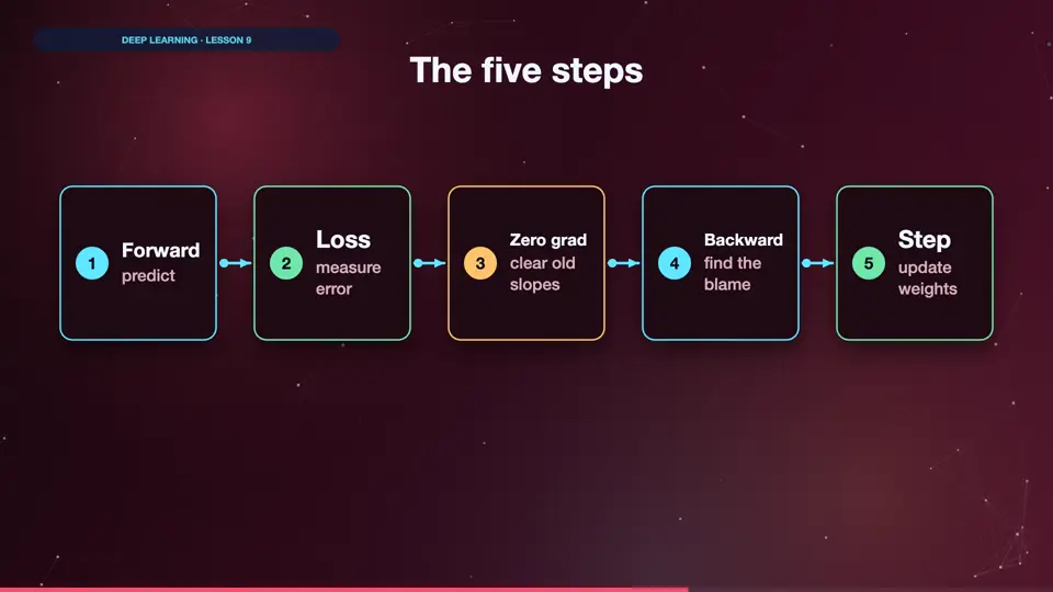
Here they are. One, forward, where the model makes predictions. Two, loss, which measures how wrong they are. Three, zero grad, which clears the old gradients. Four, backward, which computes how each weight contributed to the error. And five, step, where the optimiser nudges all of the weights. Then we repeat, millions of times. That's it. All the rest is detail.

1. Forwardpredict
2. Lossmeasure error
3. Zero gradclear old slopes
4. Backwardfind the blame
5. Stepupdate weights

Training on fashion

Let's do it for real. Fashion M N I S T holds small images of shirts, shoes, and bags, which are harder than digits. Adam is the optimiser, and cross entropy is the loss for classification. Now look at the loop, and find our five lines. Model dot train and model dot eval switch certain layers between training and testing modes. And no grad saves memory when we're only measuring. Run it. Three passes over sixty thousand images, and we're near eighty seven percent on images that it's never seen.

import torch
from torch import nn
from torch.utils.data import DataLoader
from torchvision import datasets, transforms

root = "data"
tf = transforms.ToTensor()
train = datasets.FashionMNIST(root, train=True, transform=tf)
test = datasets.FashionMNIST(root, train=False, transform=tf)
train_dl = DataLoader(train, batch_size=128, shuffle=True)
test_dl = DataLoader(test, batch_size=512)

model = nn.Sequential(nn.Flatten(), nn.Linear(784, 256), nn.ReLU(),
                      nn.Linear(256, 10))
opt = torch.optim.Adam(model.parameters(), lr=1e-3)
loss_fn = nn.CrossEntropyLoss()

for epoch in range(1, 4):
    model.train()
    for x, y in train_dl:
        loss = loss_fn(model(x), y)
        opt.zero_grad()
        loss.backward()
        opt.step()

    model.eval()
    correct = 0
    with torch.no_grad():
        for x, y in test_dl:
            correct += (model(x).argmax(1) == y).sum().item()
    print(f"epoch {epoch}  accuracy {correct / len(test):.3f}")

epoch 1  accuracy 0.834
epoch 2  accuracy 0.859
epoch 3  accuracy 0.857

Where does it go wrong?

A single accuracy number hides a lot. So let's look at which classes the model finds hard. We count the mistakes for each class, and sort them. Run it. Shirts cause the most trouble, and that makes sense, because a shirt looks a lot like a coat, or a pullover. Looking at your errors is always a good idea. It shows you where the model is confused, and whether that confusion makes any sense.

import torch
from torch import nn
from torchvision import datasets, transforms

test = datasets.FashionMNIST("data", train=False,
                             transform=transforms.ToTensor())
names = test.classes
X = test.data.float().unsqueeze(1) / 255
y = test.targets

torch.manual_seed(0)
train = datasets.FashionMNIST("data", train=True, transform=transforms.ToTensor())
dl = torch.utils.data.DataLoader(train, batch_size=128, shuffle=True)
model = nn.Sequential(nn.Flatten(), nn.Linear(784, 256), nn.ReLU(), nn.Linear(256, 10))
opt = torch.optim.Adam(model.parameters())
for _ in range(3):
    for a, b in dl:
        l = nn.functional.cross_entropy(model(a), b)
        opt.zero_grad(); l.backward(); opt.step()

with torch.no_grad():
    pred = model(X).argmax(1)
wrong = pred != y
per = [(wrong[y == i].float().mean().item(), names[i]) for i in range(10)]
for rate, name in sorted(per, reverse=True)[:4]:
    print(f"{name:<12} wrong {rate:.1%}")

Shirt        wrong 40.9%
Pullover     wrong 30.0%
Dress        wrong 25.0%
Coat         wrong 13.8%

Your turn: add a layer

Your turn. Pause here. Take the model from this lesson, and add one more hidden layer, of one hundred and twenty eight neurons, after the first. Train for three epochs. Does the accuracy change? Think about what line needs to change. Just the model definition. The training loop stays exactly the same, and that's the beauty of it. Here's one solution. The extra layer, plus a ReLU, and everything else is untouched.

from torch import nn

model = nn.Sequential(
    nn.Flatten(),
    nn.Linear(784, 256), nn.ReLU(),
    nn.Linear(256, 128), nn.ReLU(),
    nn.Linear(128, 10),
)
print(model)
print("Weights:", sum(p.numel() for p in model.parameters()))

Sequential(
  (0): Flatten(start_dim=1, end_dim=-1)
  (1): Linear(in_features=784, out_features=256, bias=True)
  (2): ReLU()
  (3): Linear(in_features=256, out_features=128, bias=True)
  (4): ReLU()
  (5): Linear(in_features=128, out_features=10, bias=True)
)
Weights: 235146

Summary