
This deep-learning tutorial will teach you how to implement a convolutional neural network using TensorFlow. The convolutional neural network is an architecture that is used for different tasks such as image classification, image recognition, and object detection.
This tutorial is focused on image classification. There are many datasets available for image classification but in this tutorial, we will use the CIFAR10 dataset. This dataset has 60,000 images that are divided into 10 classes. There are 10,000 images for each class. The data is already split into training and testing. The 50,000 images are present in the training set and 10,000 images are present in the test set. I will try my best to explain everything and to make it very simple and easy. You just have to follow the 8 steps to implement CNN for an image classification task.
Step 1: Import the required modules
import tensorflow as tf
from tensorflow.keras import datasets, layers, models
import matplotlib.pyplot as plt
Step 2: Download the CIFAR10 dataset
(train_images, train_labels), (test_images, test_labels) = datasets.cifar10.load_data()
Step 3: Normalize the data between 0 and 1
train_images, test_images = train_images / 255.0, test_images / 255.0
Step 4: Visualize the data
categories = ['airplane', 'automobile', 'bird', 'cat', 'deer',
               'dog', 'frog', 'horse', 'ship', 'truck']

plt.figure(figsize=(15,10))
for i in range(20):
    plt.subplot(4,5,i+1)
    plt.xticks([])
    plt.yticks([])
    plt.grid(False)
    plt.imshow(train_images[i])
    plt.xlabel(categories[train_labels[i][0]])
plt.show()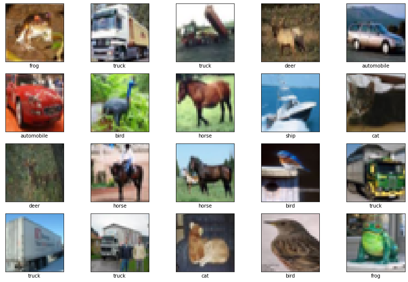
Step 5: Create a Model (Convolutional and Polling Layers)
model = models.Sequential()
model.add(layers.Conv2D(32, (3, 3), activation='relu', input_shape=(32, 32, 3)))
model.add(layers.MaxPooling2D((2, 2)))
model.add(layers.Conv2D(64, (3, 3), activation='relu'))
model.add(layers.MaxPooling2D((2, 2)))
model.add(layers.Conv2D(128, (3, 3), activation='relu'))
model.summary()
Model: "sequential"
_________________________________________________________________
 Layer (type)                Output Shape              Param #
=================================================================
 conv2d (Conv2D)             (None, 30, 30, 32)        896

 max_pooling2d (MaxPooling2D  (None, 15, 15, 32)       0
 )

 conv2d_1 (Conv2D)           (None, 13, 13, 64)        18496

 max_pooling2d_1 (MaxPooling  (None, 6, 6, 64)         0
 2D)

 conv2d_2 (Conv2D)           (None, 4, 4, 128)         73856

=================================================================
Total params: 93,248
Trainable params: 93,248
Non-trainable params: 0
_________________________________________________________________
To verify the output shape you can use this formula:
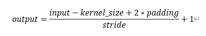
You can calculate the number of parameters using the following formula. In the formula, n and m is the height and width of a filter. l is the number of (channels/depth/number of filters) of previous layer. k is the number of filters for the current layer.
(n*m*l+1)*k
For the first convolutional layer:
n = m = 3, k = 32, l = 3 and +1 for the bias
For the second convolutional layer:
n = m = 3, k = 64, l = 32 and +1 for the bias
For the third convolutional layer:
n = m = 3, k = 128, l = 64 and +1 for the bias
Step 6: Flatten and Dense layers
Now flatten the 3D output to 1D (4*4*128 = 2048). Then feed this into dense layers to perform classification. In the first dense layer, 256 is number of neurons. In the second dense layer, that is the final layer in which 10 is the number of neurons that is equal to our number of classes.
model.add(layers.Flatten())
model.add(layers.Dense(256, activation='relu'))
model.add(layers.Dense(10))
model.summary()
Model: "sequential"
_________________________________________________________________
 Layer (type)                Output Shape              Param #
=================================================================
 conv2d (Conv2D)             (None, 30, 30, 32)        896

 max_pooling2d (MaxPooling2D  (None, 15, 15, 32)       0
 )

 conv2d_1 (Conv2D)           (None, 13, 13, 64)        18496

 max_pooling2d_1 (MaxPooling  (None, 6, 6, 64)         0
 2D)

 conv2d_2 (Conv2D)           (None, 4, 4, 128)         73856

 flatten (Flatten)           (None, 2048)              0

 dense (Dense)               (None, 256)               524544

 dense_1 (Dense)             (None, 10)                2570

=================================================================
Total params: 620,362
Trainable params: 620,362
Non-trainable params: 0
_________________________________________________________________
Step 7: Compile and train the model
model.compile(optimizer='adam',
              loss=tf.keras.losses.SparseCategoricalCrossentropy(from_logits=True),
              metrics=['accuracy'])

history = model.fit(train_images, train_labels, epochs=20,
                    validation_data=(test_images, test_labels))
Epoch 1/20 1563/1563 [==============================] - 45s 28ms/step - loss: 1.4195 - accuracy: 0.4856 - val_loss: 1.1494 - val_accuracy: 0.5867 Epoch 2/20 1563/1563 [==============================] - 46s 29ms/step - loss: 1.0238 - accuracy: 0.6414 - val_loss: 1.0582 - val_accuracy: 0.6347 Epoch 3/20 1563/1563 [==============================] - 45s 29ms/step - loss: 0.8539 - accuracy: 0.7008 - val_loss: 0.8975 - val_accuracy: 0.6839 Epoch 4/20 1563/1563 [==============================] - 45s 29ms/step - loss: 0.7399 - accuracy: 0.7391 - val_loss: 0.8157 - val_accuracy: 0.7200 Epoch 5/20 1563/1563 [==============================] - 45s 29ms/step - loss: 0.6406 - accuracy: 0.7741 - val_loss: 0.8481 - val_accuracy: 0.7137 Epoch 6/20 1563/1563 [==============================] - 47s 30ms/step - loss: 0.5620 - accuracy: 0.8028 - val_loss: 0.8181 - val_accuracy: 0.7307 Epoch 7/20 1563/1563 [==============================] - 51s 33ms/step - loss: 0.4770 - accuracy: 0.8289 - val_loss: 0.8476 - val_accuracy: 0.7324 Epoch 8/20 1563/1563 [==============================] - 51s 32ms/step - loss: 0.4012 - accuracy: 0.8573 - val_loss: 0.8897 - val_accuracy: 0.7342 Epoch 9/20 1563/1563 [==============================] - 51s 33ms/step - loss: 0.3354 - accuracy: 0.8802 - val_loss: 0.9964 - val_accuracy: 0.7101 Epoch 10/20 1563/1563 [==============================] - 49s 31ms/step - loss: 0.2755 - accuracy: 0.9018 - val_loss: 1.0710 - val_accuracy: 0.7235 Epoch 11/20 1563/1563 [==============================] - 47s 30ms/step - loss: 0.2318 - accuracy: 0.9169 - val_loss: 1.1629 - val_accuracy: 0.7213 Epoch 12/20 1563/1563 [==============================] - 47s 30ms/step - loss: 0.1966 - accuracy: 0.9315 - val_loss: 1.2877 - val_accuracy: 0.7167 Epoch 13/20 1563/1563 [==============================] - 45s 29ms/step - loss: 0.1657 - accuracy: 0.9415 - val_loss: 1.3650 - val_accuracy: 0.7203 Epoch 14/20 1563/1563 [==============================] - 49s 31ms/step - loss: 0.1472 - accuracy: 0.9472 - val_loss: 1.4356 - val_accuracy: 0.7141 Epoch 15/20 1563/1563 [==============================] - 47s 30ms/step - loss: 0.1408 - accuracy: 0.9508 - val_loss: 1.4986 - val_accuracy: 0.7142 Epoch 16/20 1563/1563 [==============================] - 51s 32ms/step - loss: 0.1217 - accuracy: 0.9583 - val_loss: 1.6737 - val_accuracy: 0.7076 Epoch 17/20 1563/1563 [==============================] - 47s 30ms/step - loss: 0.1247 - accuracy: 0.9578 - val_loss: 1.7020 - val_accuracy: 0.7114 Epoch 18/20 1563/1563 [==============================] - 47s 30ms/step - loss: 0.1114 - accuracy: 0.9618 - val_loss: 1.8628 - val_accuracy: 0.7124 Epoch 19/20 1563/1563 [==============================] - 51s 33ms/step - loss: 0.1075 - accuracy: 0.9638 - val_loss: 1.9234 - val_accuracy: 0.6992 Epoch 20/20 1563/1563 [==============================] - 47s 30ms/step - loss: 0.1014 - accuracy: 0.9658 - val_loss: 2.0329 - val_accuracy: 0.7074
Step 8: Evaluate the model and plot accuracy
plt.plot(history.history['accuracy'], label='accuracy')
plt.plot(history.history['val_accuracy'], label = 'val_accuracy')
plt.xlabel('Epoch')
plt.ylabel('Accuracy')
plt.ylim([0.5, 1])
plt.legend(loc='lower right')

test_loss, test_acc = model.evaluate(test_images,  test_labels, verbose=2)
print(test_acc)
313/313 - 3s - loss: 2.0329 - accuracy: 0.7074 - 3s/epoch - 8ms/step 0.7074000239372253
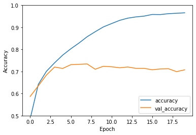
Conclusion:
After 20 epochs, the training accuracy is 96% and the validation accuracy is 70%. To increase the accuracy, you can change the parameters such as the number of filters, filter size, number of epochs, number of layers, etc. You can do many things to improve the validation accuracy.